Time-domain radio astronomy with MonetDB
The international low-frequency radio telescope LOFAR (located in The Netherlands) is one of the first telescopes to completely integrate observations with real-time computation and data storage facilities in its overall design. Signals received by thousands of antennas are locally pre-processed and digitised before they are transported over a 10Gb/s link to a remote supercomputer. There, the raw data is processed further, e.g., imaged, after which dedicated software pipelines pick up the calibrated data again to do their science.
LOFAR and the Transients Pipeline
LOFAR has several scientific working groups, but here we will restrict ourselves to the Transients Key Science Project Group and their automated transients detection software pipeline also known as the TraP.
One of the scientific goals of LOFAR and thus its Transients Pipeline (TraP) is to find transient and variable sources of astrophysical origin in the calibrated images on many timescales, ranging from seconds to years. Therefore, the telescope design (hardware and software) was such to be able to produce a calibrated image every few to about ten seconds, meaning that the TraP must be able to finish all that processing within the image cadence time. That is what time-domain astronomy is, it is like drinking water from a fire hose.
The speed of processing and data accumulation obviously depend on the number of sources, image resolution, and some other parameters, but in general the TraP builds up an archive that grows with 50TB per year. The archive contains extracted source properties, not the images themselves. Although “archive“ sounds a bit static, this is not at all the case.
Finding the right database
MonetDB showed off its power and potential (Ivanova et al. 2007) by being the only database alternative (to the commercial SQLServer) that succeeded loading and querying the SkyServer data from the Sloan optical telescope, still the largest source archive of a single telescope. This triggered and stimulated further development to meet the astronomical needs, LOFAR being the next.
The fact that MonetDB is a main-memory column store, optimised for bulk processing and complex querying makes it the primary option for data-intensive astronomical applications. Scientific queries mostly touch a few columns, whereas tables might have more than 400 columns. Even tables with over 1000 columns are not exceptional. The ease of extending its functionality with UDFs written in SQL, C, R and recently Python are other serious strengths. Furthermore, as was shown in another blog, MonetDB data vaults makes data loading of binary FITS files amazingly fast. Overall performance is orders of magnitude faster than good old row stores or not possible at all for NoSQL stores.
In this blogpost, we will carry out a real performance assessment and compare the popular row-store PostgreSQL with MonetDB by running the Transients Pipeline on both databases.
What the Transients Pipeline does
We will limit ourselves to a brief description of the TraP (the reader is referred to the public code repository and some papers giving short and in-depth descriptions of the TraP). After every observation, the measured results are added to the measurement table. After that, the freshly measured sources are cross-matched (associated) with their counterparts, i.e. the sources already known in the database but measured at previous timestamps and/or other telescope configurations. Found matches (associations) are linked together and stored in a time series table. For each known source there is a single unique entry in the catalogue table. In the meantime, the catalogue of known sources is updated and the new measurements are now included in the time series. For every image the TraP compares the list of new measurements with the existing model –a clever and fast way to immediately detect deviations and keep the number of comparisons in control. Significant deviations might be reported by alerts to the community for further investigation. Also, in this way the TraP and astronomers have easy access to the full source catalogue and time series data.
The source catalogue is expected to have about 10 million (unique) entries, while the list of individual measurements is 3 orders of magnitude larger. The catalogue maintains many statistical parameters, e.g., weighted and squared averages, variability indicators, and may be considered as a sky model. We ensure that the model and catalogue are always ready and up to date inside the database.
All this is done with about 30 SQL queries. From a database performance perspective it is very important to get acquainted with these “benchmark” queries. Will they still perform in the long term? Do they scale linearly over time as data accumulates? The only way to answer these questions is to assess query performance in reliable situations.
The queries
We cannot dive into all queries here (see tkp/db for the whole set), but I want to highlight (partly) one of them, the mother of all queries (MoQ), which is notorious because it does nearly all the work necessary. The idea behind it is that we leave the data inside the database and bring the computations to the data. It looks for counterparts between the just added new sources (in extractedsource) and the known catalogued sources (in runningcatalog), while at the same time it calculates the new statistical values for the candidate counterpart pairs. See the SQL code snippets below to get the idea.
Doing the cross-match:
    ,runningcatalog rc0
    ,image i0
WHERE i0.id = %(image_id)s
  AND ...
  AND rc0.zone BETWEEN CAST(FLOOR (x0.decl - %(beamwidths_limit)s * i0.rb_smaj) AS INTEGER)
                   AND CAST(FLOOR (x0.decl + %(beamwidths_limit)s * i0.rb_smaj) AS INTEGER)
  AND rc0.wm_decl BETWEEN x0.decl - %(beamwidths_limit)s * i0.rb_smaj
                      AND x0.decl + %(beamwidths_limit)s * i0.rb_smaj
  AND rc0.wm_ra BETWEEN x0.ra - alpha(%(beamwidths_limit)s * i0.rb_smaj, x0.decl)
                    AND x0.ra + alpha(%(beamwidths_limit)s * i0.rb_smaj, x0.decl)
  AND rc0.x * x0.x + rc0.y * x0.y + rc0.z * x0.z > COS ( RADIANS (%(beamwidths_limit)s * i0.rb_smaj))
  AND SQRT(  (rc0.wm_ra - x0.ra) * COS (RADIANS ((rc0.wm_decl + x0.decl)/2)) *
             (rc0.wm_ra - x0.ra) * COS (RADIANS ((rc0.wm_decl + x0.decl)/2)) /
             (x0.uncertainty_ew * x0.uncertainty_ew + rc0.wm_uncertainty_ew * rc0.wm_uncertainty_ew)
           + (x0.decl - rc0.wm_decl) * (x0.decl - rc0.wm_decl) /
             (x0.uncertainty_ns * x0.uncertainty_ns + rc0.wm_uncertainty_ns * rc0.wm_uncertainty_ns)
          ) < %(deRuiter)s
...
The where clause determines whether the associations are considered to be genuine when the critera are fulfilled. A candidate pair should at least lie in the same area bounded by their adjacent zones (zone is a declination strip), min and max polar coordinates RA and DEC where we have to take into account that RA (the longitude) inflates towards the poles (therefore the alpha() SQL function). The angular distance (the dot product of the Cartesian coordinates) of the pair should also lie within a multiple number of the semi-major axis of the telescope’s restoring beam. The last where clause, with the square root, is true when the distance between the counterparts weighted by their positional errors is less than a user specified value, which is related to a user-specified significant probability of the Rayleigh distribution. Let’s say it is not trivial.
The same query calculates at the same time the updated values for the statistical parameters:
,...
,rc0.datapoints + 1 AS datapoints
,(datapoints * rc0.avg_wra + x0.ra / (x0.uncertainty_ew * x0.uncertainty_ew)) /
 (datapoints * rc0.avg_weight_ra + 1 / (x0.uncertainty_ew * x0.uncertainty_ew)) AS wm_ra
,...
Because we have an association pair the number of data points for known source is incremented by one. Its weighted positional average now includes the new measurement, etc.
After this other queries follow that sort out the many-to-many relations of candidate pairs and do some other bookkeeping stuff.
Simulations and results
A realistic simulation would be to have images with about 100 sources where there might be denser regions having peaks up to 1,000 sources. These situation are typical for LOFAR, e.g., the Radio Sky Monitor (RSM). The number of images is more arbitrary, but to have the tests finished at the end of the day let’s have series of 10,000 (for low and high source density images) and 100,0000 (for low source density images).
We will simulate it, where we use the monitoring version of the TraP code and some bash scripts knitting it all together (setting the number of sources per image and the total number of images, initialising and running the tests). The scripts are in a private repository and the interested reader is kindly requested to contact the author for more information. Databases used are PostgreSQL and MonetDB. We have the SciLens cluster at our disposal where we can run the tests on a large variety of hardware configurations. Our tests were run on the rocks nodes in the SciLens cluster. Their specifications are given here, the main ones being CPU clockspeed of 3.6GHz CPU and RAM size of 16GB.
PostgreSQL version 9.3.5 was used. The default set-up is not sufficient for our purposes, we had to set some of the
configuration parameters: shared_buffer = 8G; chkp_segm = 256; chkp_timeo = 1h; chkp_compl_trg = 0.9; eff_cache_sz = 12GB.
For MonetDB we used the Oct2014-SP1 version and its default configuration (compiled with --enable-optimize option).
The graphs below show the results for MonetDB (left images) and PostgreSQL (right images). The first row of graphs shows the case of 100 sources per image and a series of 10,000 images, the second row of graphs shows the results for source densities of 1,000 and again a sequence of 10,000 images. The third rows shows the performance when we have 100 sources per image and a sequence of 100,000 images.
Horizontal axes display the image number in the sequence. The accumulated processing time for a query is shown on the vertical axes. Each query has its own curve for which the line color and style can be read in the legend. Note that the same query not necessarily has the same color and style in another graph. At first sight they might be hard to understand because they display so many queries, but what one generally wants to see is linear behaviour for each query during the whole run. Exponential growth is not good, such query execution plans are not sustainable with time.
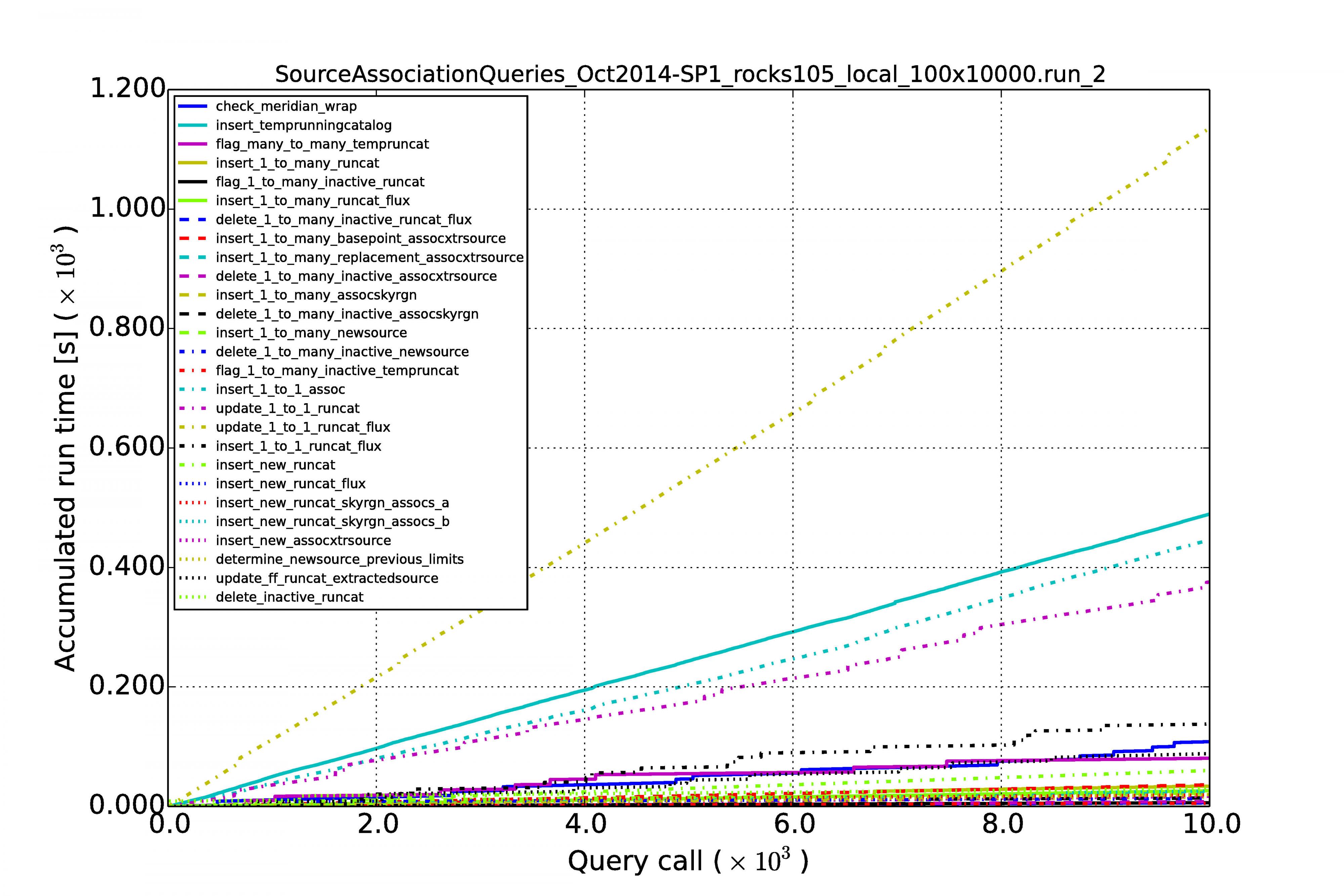
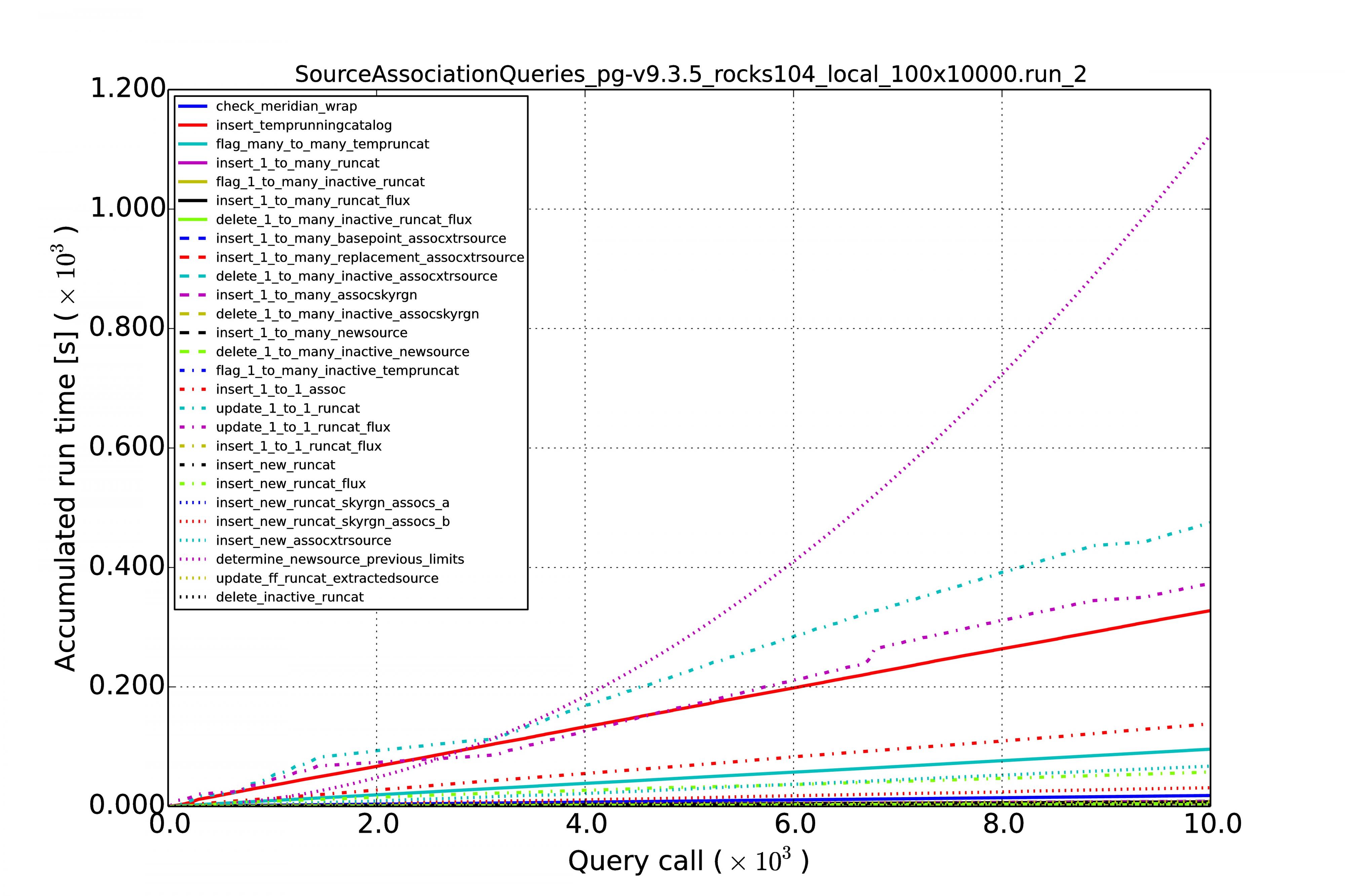
The graphs above show the results for the low source densities for a sequence of 10,000 images. (Right-click on image to enlarge.)
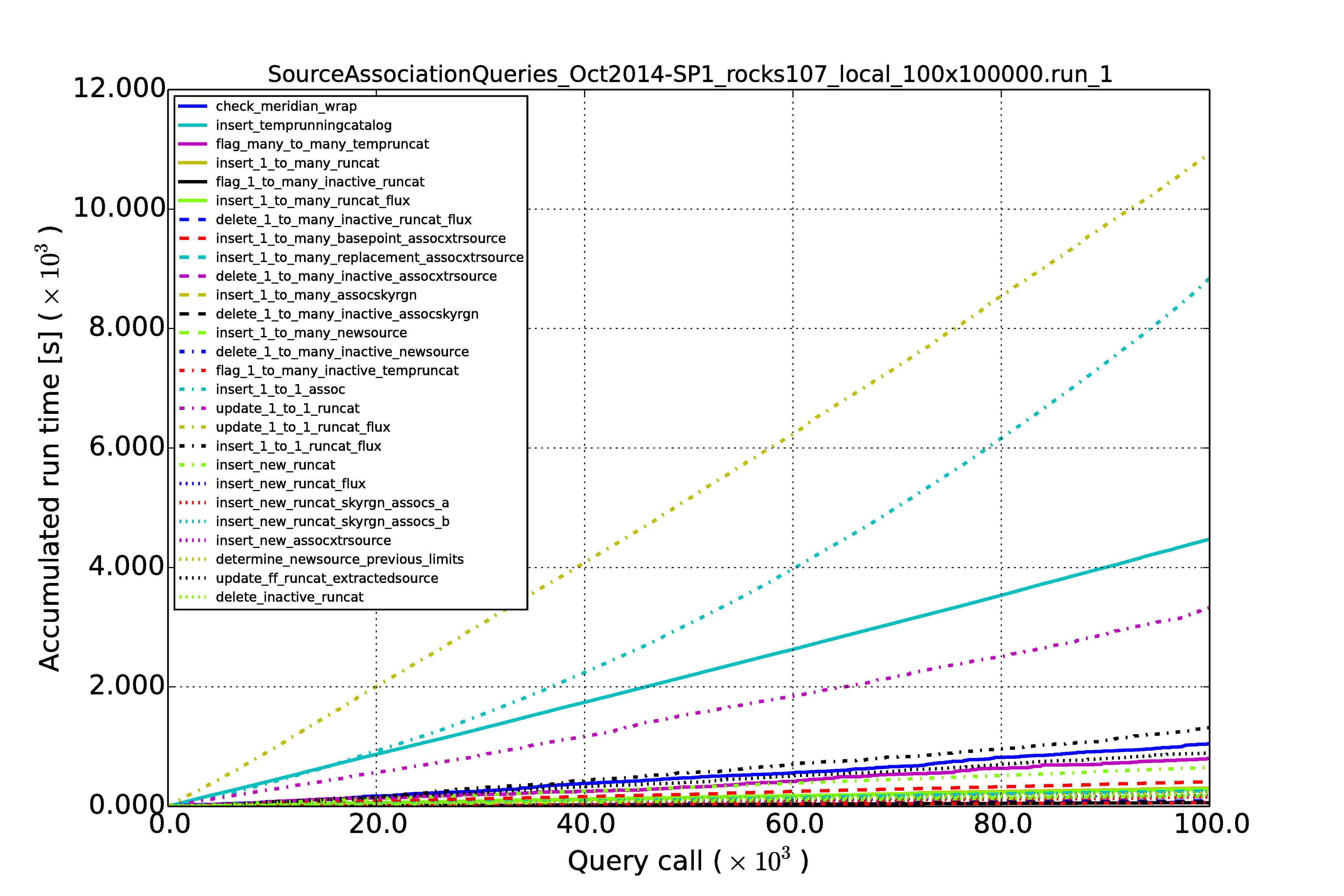
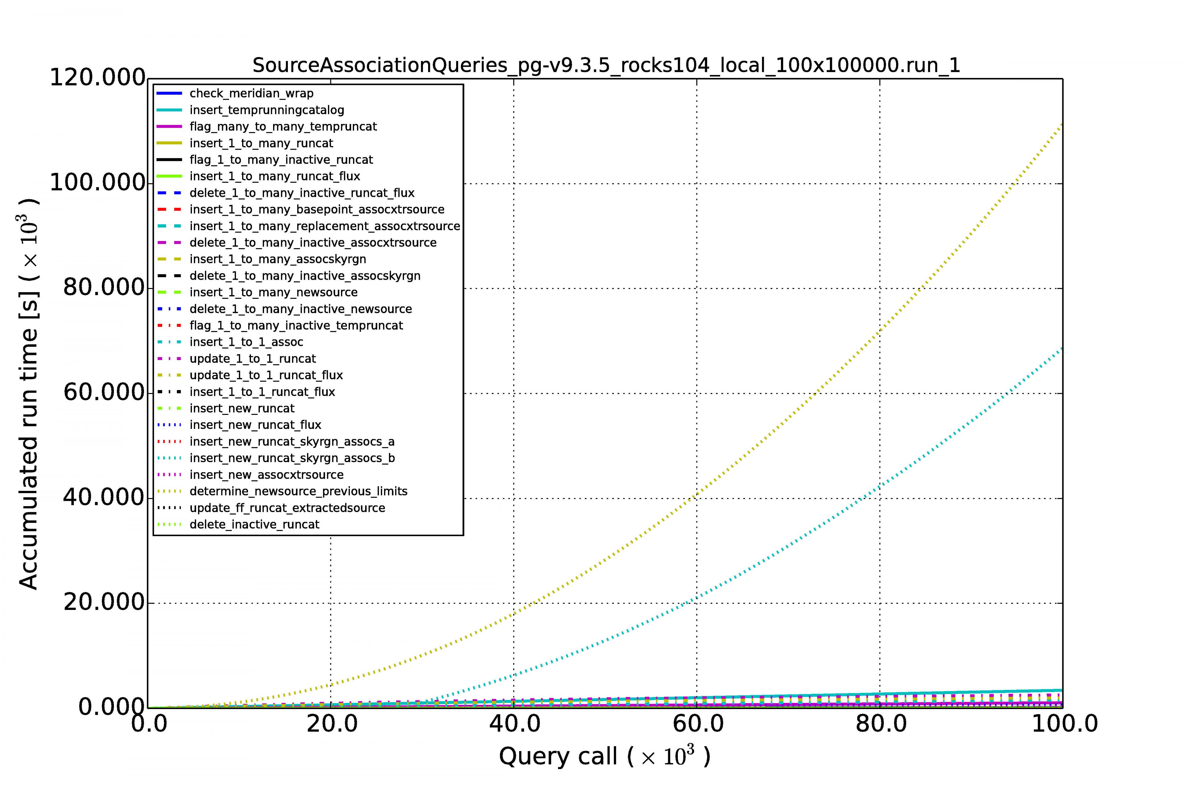
Above are the results for the low source density but now for a sequence of 100,000 images.
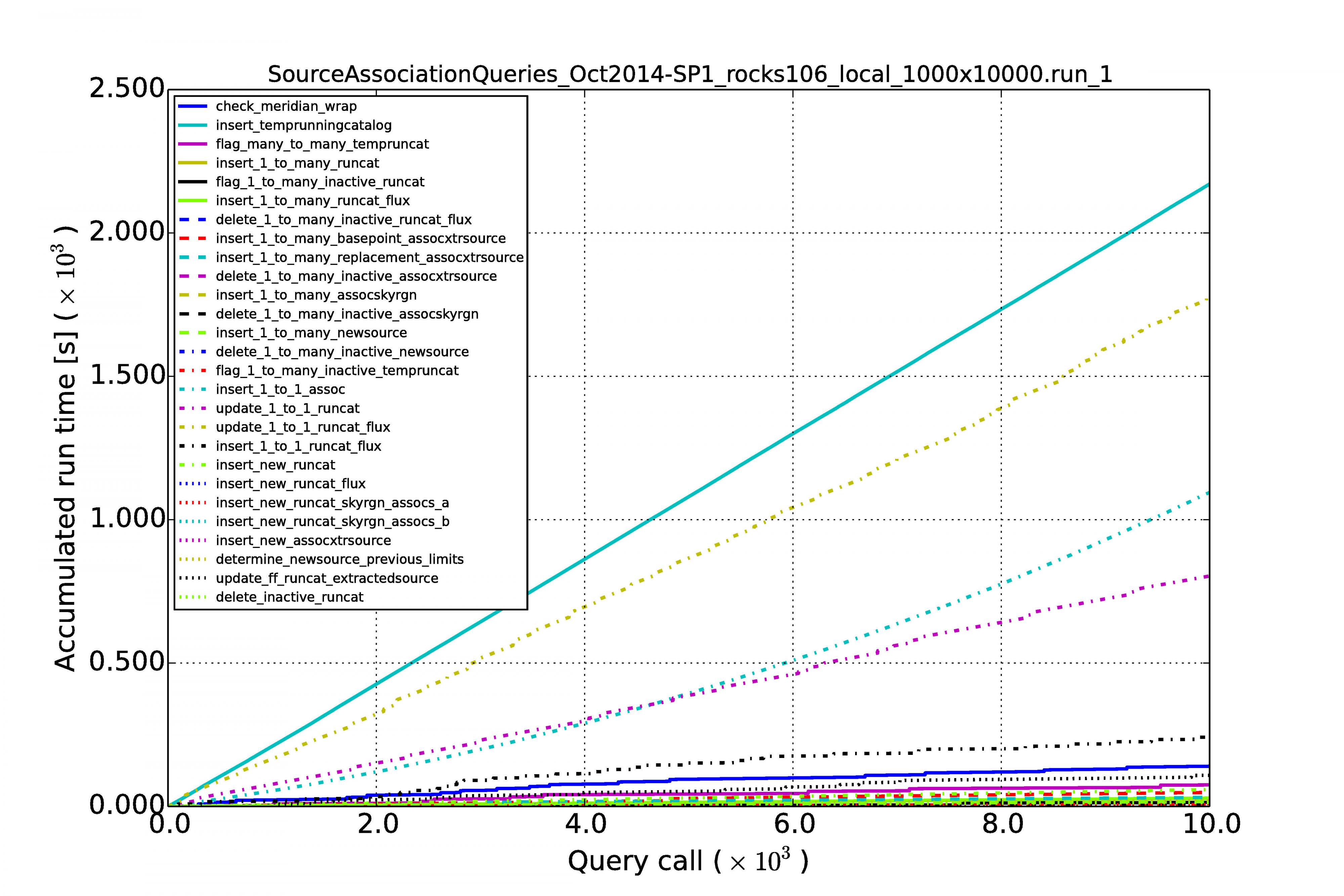
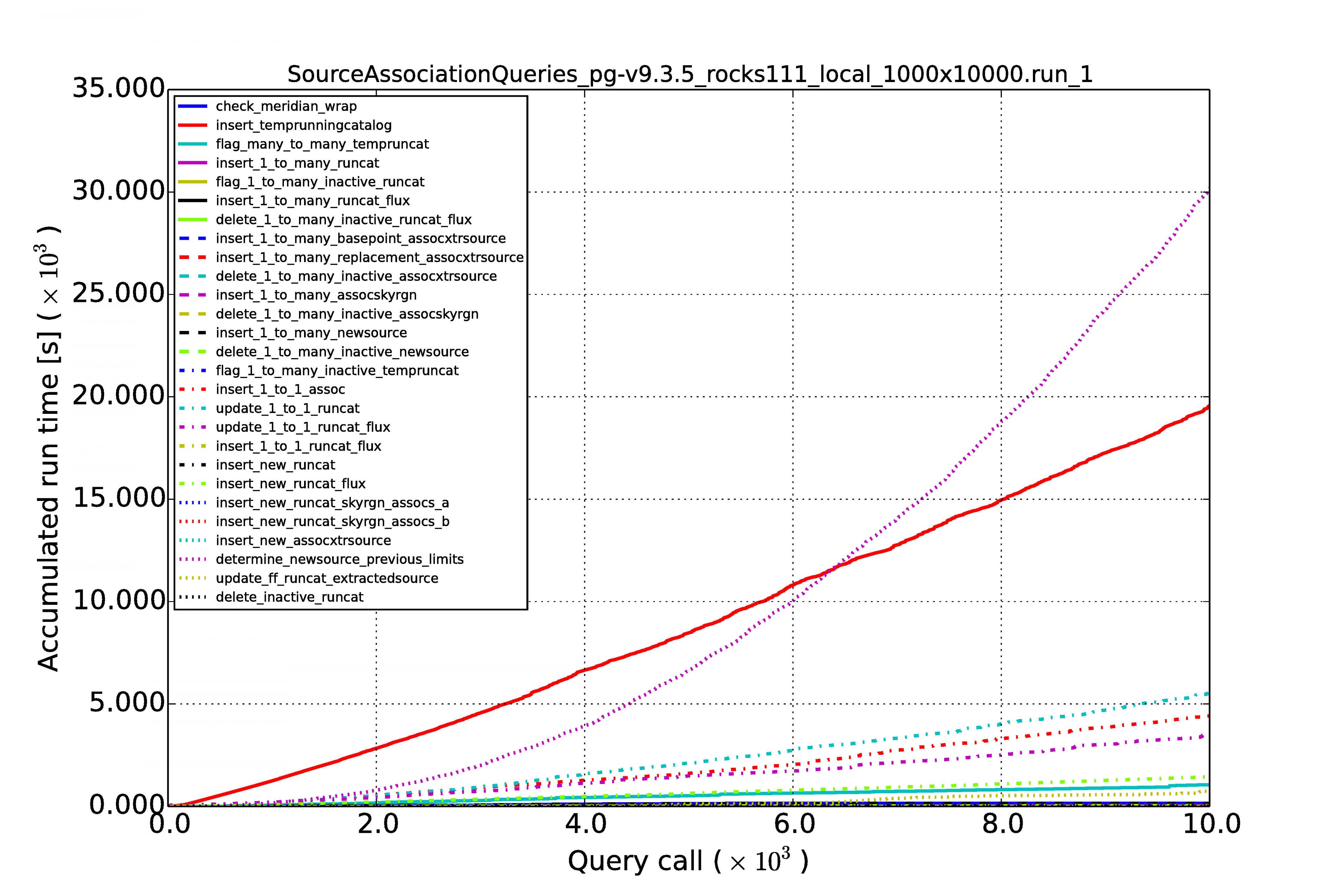
The graphs above display the results for the high source densities for a sequence of 10,000 images.
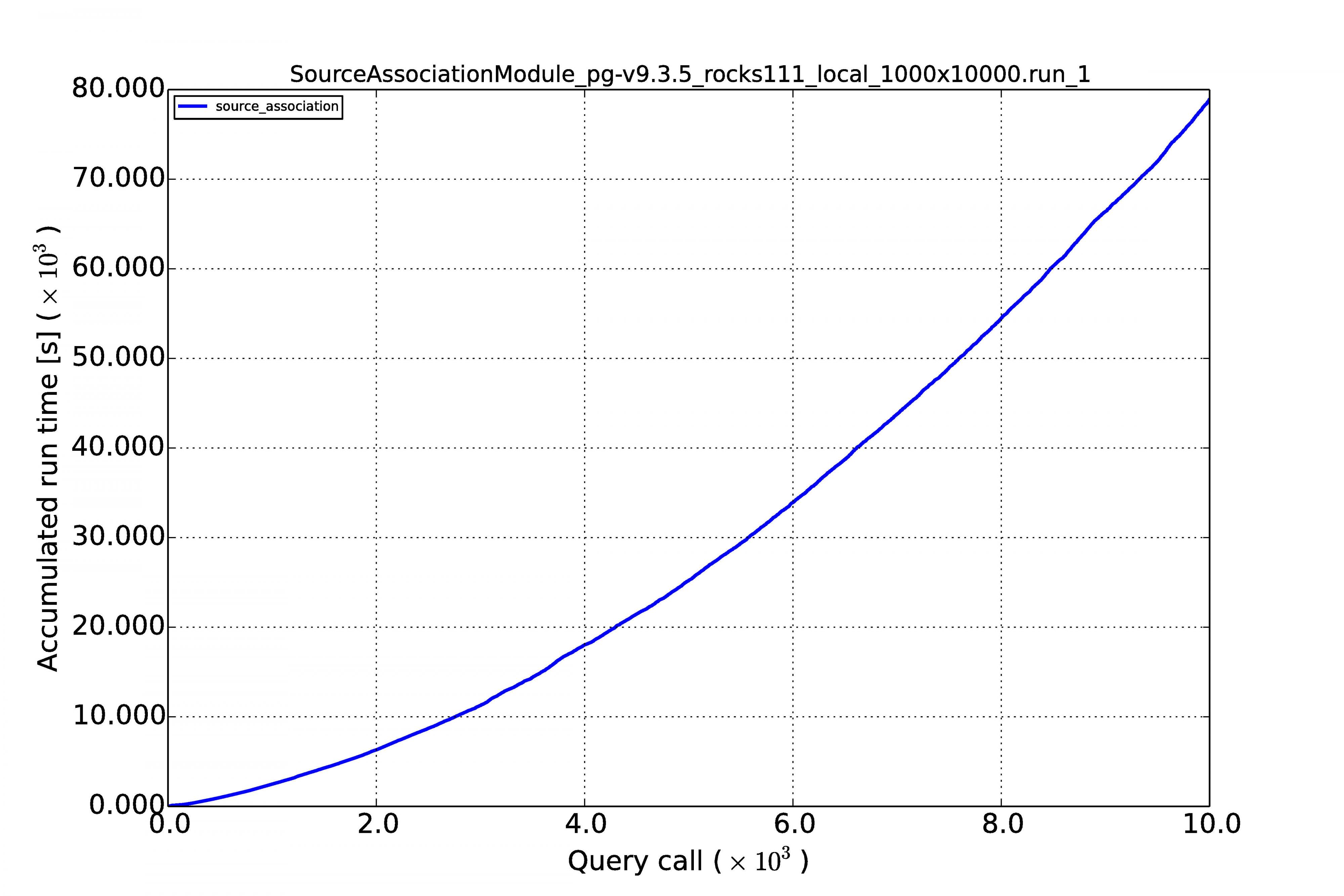
If we add all the query times spent per image the effect of linearity becomes even more visible. The following plots show the results for the sequence of 10,000 images with the high source densities of 1,000 per image.

Conclusive remarks
From the above results we can see that the performance is reasonably linear for all queries, for MonetDB at least. In the case of PostgreSQL, some queries (not the MoQ) start to grow exponentially. Apparently, the fact that the database keeps on growing, makes the row store and its query plans very sensitive to complex queries having multiple joins. The difference is not that large at low source densities for shorter image sequences, but becomes an order of magnitude at larger scales.
An important result is that the query execution time for every image (whether it is the first or last in the sequence) is constant in the case of the MonetDB column store. Our sky model is of the same size as the newly arriving sources (we never query over a whole table), making the cross-matching and other manipulations of the same order every time. This scales linearly when we increase the source density from 100 to 1,000.
We can see that for MonetDB all the source association queries run in 80% of the image cadence time, which is acceptable.
Prospects
Although these results are promising, the current database schema cannot handle the scale of source densities which reach into the 100,000s. We believe that enhancing the database kernel with kd-tree functionality can open up the time domain for optical astronomy as well, and especially the scientific discoveries to be made by the future optical instruments, e.g., MeerLICHT, BlackGEM, LSST, and the world’s largest radio telescope SKA. They will surely benefit from this.