Voter Classification using MonetDB/Python
In a previous blogpost we introduced MonetDB/Python. Using MonetDB/Python, users can execute their own vectorized Python functions within MonetDB without having to worry about slow data transfer. In this post we only really showcased simple Python functions, such as computing the quantile or summing up a set of integers. We don’t really need Python UDFs to do these simple operations. We can easily do them using SQL as well.
In this blogpost, we will go a step further and do something we really would not want to do in SQL.
We will use MonetDB/Python to do everything that is needed to train a classifier on a dataset.
We will preprocess the data and then divide the data into a train and test set.
We will train the classifier on the train set, and then test the trained classifier on the test set using the
sklearn package. All this without the data ever leaving MonetDB.
Voter Classification
In our example, we are going to perform classification of voters in North Carolina. We are going to try to predict which party voters will vote for in the upcoming election based on the previous election results.
For this, we have obtained two separate datasets that are publicly available from here.
- The first dataset,
ncvoters, contains the information about the individual voters. This is a dataset of 7.5M rows with each row containing information about the person voting. There are 96 columns in total, but for simplicity we will only look at county, precinct, gender, ethnicity and age. Note that we do not know who each person actually voted for, as this information is not publicly available. - The second dataset,
precinct_votes, contains the voting information for each precinct. So how many people in each precinct voted for Obama, and how many voted for Romney. This dataset has 2751 rows, one for each precinct. This is publicly available information.
Our plan is to combine these two datasets to try to classify each of the voters. We know the voting records of a precinct, and we know in which precinct each person voted, so we can try and guess who they voted for based on that information.
Preprocessing
First, we will have to combine the two datasets together. These are stored as two separate tables in our database,
ncvoters and precinct_votes. This is where a database comes in handy, as we can simply join the
two tables on the county + precinct combination (we need this combination because there are multiple precincts
with the same name, but in different counties). We can also immediately filter out every person that did not vote
(this is stored in the column ncvoters.status).
CREATE TABLE ncvoters_joined AS
    SELECT republican_percentage, county, precinct, sex, race, ethnicity, age
      FROM precinct_votes INNER JOIN ncvoters
        ON ncvoters.precinct = precinct_votes.precinct
       AND ncvoters.county = precinct_votes.county
     WHERE ncvoters.status = 'A'
      WITH DATA ;
Now we have the joined table of all the voters stored in the ncvoters_joined table. Let’s take a look at a
sample from this table.
SELECT * FROM ncvoters_joined SAMPLE 5;
| republican_percentage | county | precinct | sex | race | ethnicity | age |
|---|---|---|---|---|---|---|
| 0.503355704698 | COLUMBUS | P07 | M | W | NL | 80 |
| 0.400442477876 | CRAVEN | N5 | F | B | NL | 43 |
| 0.666293393057 | JOHNSTON | PR28 | M | W | NL | 27 |
| 0.210502072778 | NEW HANOVER | W27 | M | B | NL | 63 |
| 0.650045745654 | WAKE | 19-10 | F | B | NL | 40 |
Now we have a table that contains the relevant columns. In addition, we have for each person the voting records of
the precinct he lives in, stored in the republican_percentage column. This is the percentage of people who voted
for Romney in the 2012 election in that precinct.
Before we start classification, we first have to do some preprocessing. As we can see, all of these columns are stored as STRING. However, the classifier we will use only works with numerical values. Thus we will need to convert these STRING columns to INT columns. This is where MonetDB/Python comes in handy. We can write a Python function that does the preprocessing for us.
CREATE FUNCTIONvoter_preprocess (
    republican_percentage DOUBLE, county STRING, precinct STRING,
    sex STRING, race STRING, ethnicity STRING, age INT)
RETURNS TABLE (republican_percentage DOUBLE, county INT, precinct INT,
               sex INT, race INT, ethnicity INT, age INT)
LANGUAGE PYTHON
{
    from sklearn import preprocessing
    result_columns = dict ()

    # loop over all the columns
    for key in _columns.keys():
        if _column_types[key] == 'STRING' :
            # if the column is a string, we transform it
            le = preprocessing.LabelEncoder()
            # fit the labelencoder on the data
            le.fit(_columns[key])
            # apply the labelencoder and store the result
            result_columns[key] = le.transform(_columns[key])
        else:
            # if the column is not a string, we don't need to do anything
            result_columns[key] = _columns[key]
    return result_columns
};
We can use the LabelEncoder from the sklearn library to convert STRING columns into INTEGER columns.
The LabelEncoder assigns numeric classes to every STRING value, so that every unique STRING value has a
different class.
In this example we are using two special parameters, _columns and _column_types. _columns is a (key, value)
dictionary that contains all the input columns. We use this dictionary so we can conveniently loop over all the
input columns. _column_types is a (key, value) dictionary that contains the SQL types of the input columns;
allowing us to look at the underlying SQL type of each column.
We can then call this function on our joined table to create the preprocessed table.
CREATE TABLE ncvoters_preprocessed AS
    SELECT *
      FROM voter_preprocess( (SELECT * FROM ncvoters_joined) )
      WITH DATA ;
Now we have converted all strings to categorical integer values and placed their values in the ncvoters_preprocessed
table. Let’s take a look at the table.
SELECT * FROM ncvoters_preprocessed SAMPLE 5;
| republican_percentage | county | precinct | sex | race | ethnicity | age |
|---|---|---|---|---|---|---|
| 0.693446088795 | 17 | 155 | 0 | 6 | 2 | 20 |
| 0.757894736842 | 22 | 1202 | 1 | 6 | 1 | 26 |
| 0.183315038419 | 31 | 602 | 0 | 1 | 2 | 19 |
| 0.00658761528327 | 33 | 603 | 1 | 1 | 1 | 79 |
| 0.731428571429 | 61 | 1407 | 0 | 6 | 1 | 75 |
Train/Test Split
Before we can begin our classification, we will need to divide our dataset into a train and test set. We can then use the train set to train the classifier, and the test set to verify how good the classifier is.
First, we add a unique id number to our table so we can easily identify the rows.
ALTER TABLE ncvoters_preprocessed ADD id INTEGER NOT NULL AUTO_INCREMENT ;
Now we need to decide whether or not we want to include certain rows in the train set, or place them in the test set. Because we have a very large dataset of about 5.7 million voters, we will only use 5% of the dataset as our train indices. We again use MonetDB/Python to split the data into a train/test set.
CREATE FUNCTION voter_split (precinct INT, id INT)
RETURNS TABLE (id INT, train BOOLEAN)
LANGUAGE PYTHON
{
    count = len(id)
    # generate the indices
    indices = numpy.arange(count)
    # shuffle the indices
    numpy.random.shuffle(indices)
    # assign 5% of the values to the train set
    train_indices = indices[: int (count * 0.05)]
    # create a boolean array that specifies for each value if it belongs to the train/test set
    train_set = numpy.zeros(count, dtype=numpy.bool)
    train_set[train_indices] = True
    return [id, train_set]
};
We can then use this function to create the train/test table as follows.
CREATE TABLE train_set AS
    SELECT *
      FROM voter_split( (SELECT precinct, id FROM ncvoters_preprocessed) )
      WITH DATA ;
Now we have a table train_set which contains for each row whether or not it belongs to the train set.
Let’s take a look at the table.
SELECT * FROM train_set SAMPLE 5;
| id | train |
|---|---|
| 5396917 | false |
| 4062001 | false |
| 2288450 | true |
| 2939365 | false |
| 579760 | false |
We can use this table to form the actual train or test set by joining it with the ncvoter table on the row identifier.
Training
Now we can do the actual training of the data. As mentioned previously, we will use the RandomForestClassifier from
the sklearn package. The only problem we have now is that we do not know the true classes of the voters.
Instead, all we know is the percentage of people that voted Republican or Democrat in a given precinct.
We will use this information to generate random classes for each person. We will randomly assign every voter a class of either ‘Democrat’ or ‘Republican’, weighted by the percentage of people that voted for a specific party in the precinct they live in. Consider a precinct in which 70% of the people voted for Romney and 30% voted for Obama. Each voter in that precinct has a 70% chance of being classified as a Republican voter, and a 30% chance of being classified as a Democrat voter.
After generating the classes we can do the actual fitting on our features, which are county, precinct, sex, race, ethnicity and age.
After we have fitted the classifier, we need to be able to use it for predicting on our test set. For this, we need
to be able to store our classifier somewhere and then access it in our voter predict function. For this, we can use
the pickle package provided by Python. Using this package, we can convert arbitrary Python objects, such as our
classifier, into strings and store them in the database in a STRING field.
CREATE FUNCTION voter_train (
    republican_percentage DOUBLE, county INT, precinct INT,
    sex INT, race INT, ethnicity INT, age INT)
RETURNS TABLE (cl_name STRING, cl_obj STRING)
LANGUAGE PYTHON
{
    import cPickle
    count = len(county)
    from sklearn.ensemble import RandomForestClassifier
    clf = RandomForestClassifier(n_estimators=10)

    # randomly generate the classes
    random = numpy.random.rand(count)
    classes = numpy.zeros(count, dtype='S10')
    classes[random < republican_percentage] = 'Republican'
    classes[random > republican_percentage] = 'Democrat'

    # exclude republican_percentage from the feature set
    del _columns['republican_percentage']

    # construct a 2D array from the features
    data_array = numpy.array([])
    for x in _columns.values():
        data_array = numpy.concatenate((data_array, x))
    data_array.shape = (count, len(_columns.keys()))

    # train the classifier
    clf.fit(data_array, classes)

    # export the classifier to the database
    return dict (cl_name="Random Forest Classifier", cl_obj=cPickle.dumps(clf))
};
To train the classifier on the training set and store it in the Classifiers table in our database we run
the following SQL query. Note how we join the ncvoters_preprocessed table with the train_set table to obtain
the rows that belong to our train set.
CREATE TABLE Classifiers AS
    SELECT *
      FROM voter_train(
       (SELECT republican_percentage, county, precinct, sex_code,
               race_code, ethnic_code, birth_age
          FROM ncvoters_preprocessed INNER JOIN train_set
            ON train_set.id=ncvoters_preprocessed.id
          WHERE train_set.train=true) )
      WITH DATA ;
Testing
Now we have successfully trained our classifier, all that remains for us is to use it to predict the classes of
all the voters in the test set. Our prediction takes as input the features of the test set, and outputs the class
for each row (either Democrat or Republican). We load the classifier from the database using a loopback query.
These queries allow us to query the database from within Python. We can use loopback queries by using
_conn object that is passed to every MonetDB/Python function.
CREATE FUNCTION voter_predict (
    county INT, precinct INT, sex INT, race INT,
    ethnicity INT, age INT, id INT)
RETURNS TABLE (id INT, prediction STRING)
LANGUAGE PYTHON
{
    # don't use id for prediction
    del _columns['id']

    # load the classifier using a loopback query
    import cPickle
    # first load the pickled object from the database
    res = _conn.execute("SELECT cl_obj FROM Classifiers WHERE cl_name = 'Random Forest Classifier';")
    # Unpickle the string to recreate the classifier
    classifier = cPickle.loads(res['cl_obj'][0])

    # create a 2D array of the features
    data_array = numpy.array([])
    for x in _columns.values():
        data_array = numpy.concatenate((data_array, x))
    data_array.shape = (len(id), len(_columns.keys()))

    # perform the actual classification
    result = dict ()
    result['prediction'] = classifier.predict(data_array)
    result['id'] = id
    return result
};
To run our prediction, we need to obtain the test set. We can do this by joining on the train_set table again.
CREATE TABLE predicted AS
    SELECT *
      FROM voter_predict(
        (SELECT county, precinct, sex, race, ethnicity, age, ncvoters_preprocessed.id
           FROM ncvoters_preprocessed
          INNER JOIN train_set
             ON train_set.id=ncvoters_preprocessed.id
          WHERE train_set.train=false) )
      WITH DATA ;
Now the predicted values for each row are in the predicted table. Let’s take a look at the final table.
SELECT * FROM predicted SAMPLE 5;
| id | prediction |
|---|---|
| 3591641 | Democrat |
| 4253721 | Republican |
| 3310520 | Democrat |
| 3959994 | Republican |
| 1675613 | Republican |
We have successfully used a classifier to predict the values for this dataset. Now we can use the predicted values to verify our classifier, classify more data using our classifier or other fun stuff. The possibilities are endless.
Performance
In the last blogpost we made a big deal about the performance of MonetDB/Python compared to other databases and Python data storage solutions. But then we used a small toy benchmark to test our performance compared to these other systems. It would perhaps be more interesting to test the performance of MonetDB/Python using a more realistic example.
For this benchmark, we ran the entire voter classification chain as described in the above blog post on the
full dataset. For the pure python solutions (NumPy binary files, PyTables, PandasCSV), we used
the Pandas package to perform the initial joins/filtering operations. The database solutions (Postgres, SQLite, MySQL) each perform the filter/join operations themselves using SQL before loading the data into Python.
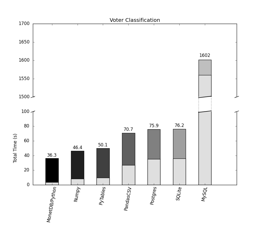
The results of the benchmark are displayed in the above figure. The numbers display the total runtime of the voter classification chain. The gray bars indicate the time spent loading the data into Python.
We can see that MonetDB/Python is still significantly faster than the alternative database solutions. However, the difference between MonetDB/Python and the alternative database solutions is smaller than in the quantile benchmark we performed last time.
The reason for this is that we spend significantly longer actually performing the operations in Python in this benchmark. In the previous benchmark we only computed the quantile, which is a relatively simple operation. In this benchmark we perform a long chain of more complex operations to classify the data.
We can see that MonetDB/Python still spends significantly less time loading the data than alternative database solutions (as displayed in the light-gray bar in the graph), however, this does not make an impact that is as pronounced as in the quantile benchmark. Rather than being forty times faster, it’s only twice as fast as the alternative database solutions.
Except for MySQL, of course.
About the Author
Mark Raasveldt is a PhD student at the CWI. If you have any questions regarding this blogpost, you can contact him at m.raasveldt@cwi.nl.