Embedded Python
This feature is outdated and has security vulnerabilities.
Python is one of the most popular languages in Data Science. It is a flexible scripting language that is easy to use and has a large amount of available statistical libraries. When we're doing statistical analysis in Python, we naturally need data accessible to us in Python in some way. And what better place to keep data than in a database.
Previously when you wanted to combine MonetDB and Python, you had to use the Python MAPI client. This client suffers from very low transfer speeds because it uses sockets. If you want to execute Python functions on larger data sets this low transfer speed quickly grows out of control.
This is why we are now introducing MonetDB/Python, in which we allow users to create their own Python functions as they would create SQL functions. The embedded Python functions can then be used within SQL statements. We show that our new method of making data available to Python analyses is faster than competing solutions.
By using NumPy arrays, which are essentially Python wrappers for C arrays, our Embedded Python implementation can transfer data from MonetDB to Python without unnecessarily copying the data, which leads to extremely fast transfer speeds. In addition, Embedded Python supports mapped operations, which allows you to run Python functions in parallel within SQL queries. Combined with the NumPy/SciPy libraries, which contain very efficient C implementations of numerous statistical and analytical functions, Embedded Python matches the speed of native SQL functions, while offering all the flexibility and ease of use of the Python scripting language. In addition, you can load any of the numerous available Python modules and use them.
Embedded Python works by creating a SQL Function that contains the Python code to be run. A simple function that multiplies the input by two is as follows.
CREATE FUNCTION python_times_two(i INTEGER) RETURNS INTEGER LANGUAGE PYTHON {
    return i * 2
};
After creating this function, we can use it in a SQL query as follows.
CREATE TABLE integers(i INTEGER);
INSERT INTO integers VALUES (1), (2), (3), (4), (5);

sql> SELECT python_times_two(i) AS result FROM integers;
+------+
| %1   |
+======+
|    6 |
|    7 |
|    8 |
|    9 |
|   10 |
+------+
Data Input
Now you might be wondering what exactly i is in this function. As we have mentioned previously, we are using NumPy for converting between MonetDB and Python. The exact type of i depends on the input; if the input contains a NULL value, i will be a MaskedArray, otherwise i will be a regular one-dimensional NumPy array. The dtype of the array depends on the type specified in the SQL function. In this example the specified type is INTEGER, which corresponds to a dtype of numpy.int32. Below is a table that contains the exact types for every possible input value:
| INPUT    | DTYPE            |
| -------- | -----------------|
| BOOLEAN  | numpy.int8       |
| TINYINT  | numpy.int8       |
| SMALLINT | numpy.int16      |
| INTEGER  | numpy.int32      |
| BIGINT   | numpy.int64      |
| REAL     | numpy.float32    |
| FLOAT    | numpy.float64    |
| HUGEINT  | numpy.float64    |
| STRING   | numpy.object [1] |
Creating Tables using Python Data
We can also use the embedded Python to create tables or insert data into existing tables. Consider the following function.
CREATE FUNCTION python_table()
RETURNS TABLE(name STRING, country STRING, age INTEGER)
LANGUAGE PYTHON {
    result = dict()
    result['name'] = ['Henk', 'John', 'Elizabeth']
    result['country'] = ['NL', 'USA', 'UK']
    result['age'] = [25, 30, 33]
    return result
};
This returns a table with three columns. We can then create an actual table in our database as follows.
CREATE TABLE people AS
  SELECT * FROM python_table()
  WITH data;

sql> SELECT * FROM people;
+-----------+---------+------+
| name      | country | age  |
+===========+=========+======+
| Henk      | NL      |   25 |
| John      | USA     |   30 |
| Elizabeth | UK      |   33 |
+-----------+---------+------+
Naturally this is only a toy example that takes no input and simply returns a constant table. Perhaps a more useful example is the following function.
CREATE FUNCTION random_integers(low INTEGER, high INTEGER, amount INTEGER)
RETURNS TABLE(value INTEGER)
LANGUAGE PYTHON {
    return numpy.random.randint(low, high, size=(amount,))
};
This function generates a table with amount entries, where each entry is a random integer between low and high.
We can then use the function to generate a table of 5 integers with a value between 0 and 10 as follows.
sql> SELECT * FROM random_integers(0, 10, 5);
+------+
| %1   |
+======+
|    4 |
|    5 |
|    8 |
|    4 |
|    2 |
+------+
Filtering Data
We can use an embedded Python function in the WHERE clause to pick which rows to include in the result set.
Consider the following function that checks, for every string in a column, if a given string (needle) is a part
of that string (haystack).
CREATE FUNCTION python_strstr(strings STRING, needle STRING)
RETURNS BOOLEAN
LANGUAGE PYTHON {
    return [needle in haystack for haystack in strings]
};
We can now use this function to select all people with the letter n in their name.
sql> SELECT * FROM people WHERE python_strstr(name, 'n');
+-----------+---------+------+
| name      | country | age  |
+===========+=========+======+
| Henk      | NL      |   25 |
| John      | USA     |   30 |
+-----------+---------+------+
Aggregating Data
Finally, we can use an embedded Python function for computing aggregates. The syntax for creating an aggregate is as follows.
CREATE AGGREGATE python_aggregate(val INTEGER)
RETURNS INTEGER
LANGUAGE PYTHON {
    try:
        unique = numpy.unique(aggr_group)
        x = numpy.zeros(shape=(unique.size))
        for i in range(0, unique.size):
            x[i] = numpy.sum(val[aggr_group==unique[i]])
    except NameError:
        # aggr_group doesn't exist. no groups, aggregate on all data
        x = numpy.sum(val)
    return(x)
};
This is a simple aggregate that sums the integers for each group or when no groups are defined for all values. We can then use the aggregate just as we would use a SQL aggregate.
CREATE TABLE grouped_ints(value INTEGER, groupnr INTEGER);
INSERT INTO grouped_ints VALUES (1, 0), (2, 1), (3, 0), (4, 1), (5, 0);

sql> SELECT groupnr, python_aggregate(value) FROM grouped_ints GROUP BY groupnr;
+---------+------+
| groupnr | %1   |
+=========+======+
|       0 |    9 |
|       1 |    6 |
+---------+------+
As you can see, this produces output equivalent to the SQL statement SUM(). If you look at the source code you will see the usage of a hidden parameter aggr_group. Note that parameter aggr_group is only created when a GROUP BY is used in the SQL query. This parameter is passed to aggregates and contains a NumPy array of the group numbers for each tuple. In the above example, aggr_group contains the numbers [0, 1, 0, 1, 0]. We then use the group numbers of each tuple to compute the aggregate value for each group.
Note also that aggr_group will always be a one dimensional array containing the group numbers, even if we do a GROUP BY over multiple columns, as in the below example.
CREATE TABLE grouped_ints(value INTEGER, groupnr INTEGER, groupnr2 INTEGER);
INSERT INTO grouped_ints VALUES (1, 0, 0), (2, 0, 0), (3, 0, 1), (4, 0, 1), (5, 1, 0), (6, 1, 0), (7, 1, 1), (8, 1, 1);

sql>SELECT groupnr, groupnr2, python_aggregate(value) FROM grouped_ints GROUP BY groupnr, groupnr2;
+---------+----------+------+
| groupnr | groupnr2 | %1   |
+=========+==========+======+
|       0 |        0 |    3 |
|       0 |        1 |    7 |
|       1 |        0 |   11 |
|       1 |        1 |   15 |
+---------+----------+------+
MonetDB transparently handles multiple groups for aggregates. In this example aggr_group will be a single array
containing the values [0, 0, 1, 1, 2, 2, 3, 3].
Performance
To keep in with tradition, we will use embedded Python to compute quantiles. We can do this efficiently using the numpy.percentile function. We will compare our embedded Python implementation against various other ways of loading data into Python and then executing the numpy.percentile function on the data, as well as some other non-Python ways of computing the quantile. In our example, we are using a single table containing 1 GB of integer values (250M values).
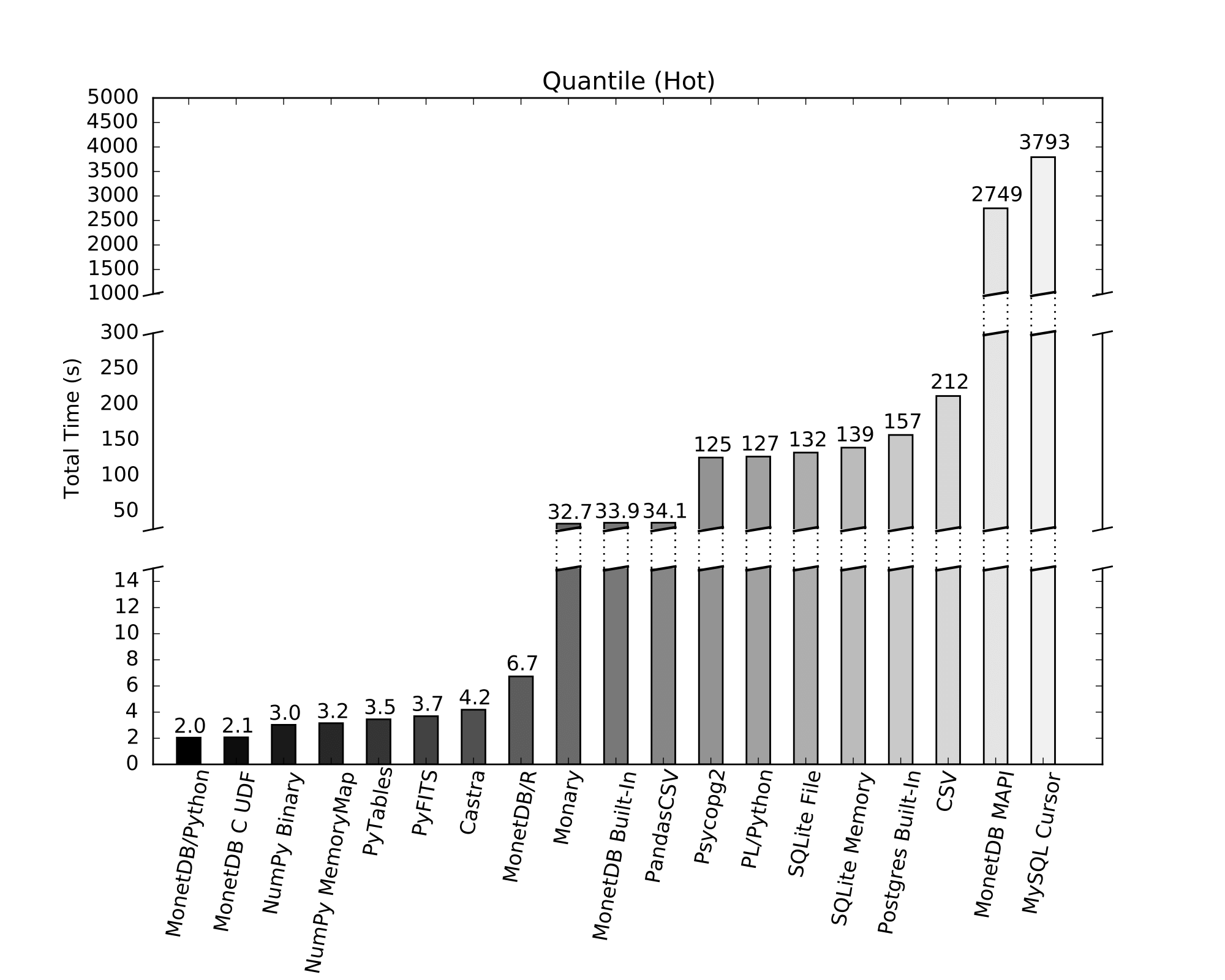
- "MonetDB/Python": this is our implementation, using
numpy.percentileon the data within a MonetDB table. MonetDB uses memory mapping to load the data into memory very quickly, and because of our zero-copy transfer into Python there is no additional overhead cost for transferring this data into Python. - "MonetDB C UDF": computes the quantile in MonetDB using a C UDF. We computed the quantile using Quickselect.
- "NumPy Binary": uses
numpy.load()to load the data into a NumPy array from a NumPy binary file. This is a very fast way of loading data into Python, because we are directly mapping a binary file into memory we do not have to do any decoding. - "NumPy MemoryMap": uses
numpy.memmap()to load the data into a NumPy array from a NumPy binary file. This has similar performance to NumPy binary files. - "PyTables": loads the data using
tables.open_file(). This is fast because it loads a binary file directly into a NumPy array. - "PyFITS": uses
pyfits.open()to load the data from into a NumPy array from a.fitsfile. - "castra": is a column-store database created entirely in Python. This uses Python pickling to load the database file as a Python object from an encoded string. This has some additional overhead.
- "MonetDB/R": uses the MonetDB/R plugin, using the native R quantile function instead of the
numpy.percentilefunction. The MonetDB/R extension does not use zero-copy transferring, which means there is extra overhead of copying the data once. In addition, it seems thenumpy.percentile()function is faster than thequantile()function in R. - "Monary": is a connector for MongoDB that is optimised for use with NumPy.
- "MonetDB Built-In": uses the built-in SQL
quantile()function in MonetDB. This function does not use a very efficient algorithm for computing the quantile, which is why it takes a while. - "PandasCSV": uses the
read_csv()function from thepandaslibrary to load the data. This is an efficient C implementation of a CSV loader. However, we still need to decode the CSV and convert it into integer values, which means the loading takes a while. - "Psycopg2": loads the data into Python using
psycopg2, the default Python connector for Postgres, and then usenumpy.percentile()to compute the quantile. This is slow because it constructs individual Python objects for every integer. - "PL/Python": loads the data from a Postgres table using
plpy.cursor()in a PL/Python function. This is slow because it loads the data as Python objects. There is also additional overhead from Postgres having to first gather all the relevant integer into a single array, as it is a row store database. - "SQLite": calls
SELECT * FROM tableto load the data from SQLite into Python, using the built-in sqlite3 module. This implementation uses Python objects for integers instead of NumPy arrays, which carry a lot of additional overhead with regards to loading as we have to construct 250 million Python integer objects (which each have to be malloc'd individually). - "Postgres Built-In": performs the quantile computation using the built-in
percentile_contaggregate, with Postgres tuned for Data Warehousing usingpgtune. - "CSV": uses the built-in Python
csvlibrary to load the data into a NumPy array. This is much less efficient than pandas'load_csv()library as it constructs Python objects. In addition, the CSV loader is written in pure Python which carries additional overhead. - "MonetDB MAPI": uses the current MonetDB Python client to load the data into Python. This is extremely slow because data has to be serialised over sockets.
- "MySQL Cursor": loads the data into Python using the MySQL Python Connector. This is extremely slow because it sends the data to Python one row at a time.
Start-up
You need to explicitly enable Python integration during server startup using the following commands if you are using
the monetdbd daemon.
monetdb stop pytest
monetdb set embedpy=true pytest
monetdb start pytest
Or the following command if you are running mserver5.
mserver5 --set embedded_py=true
In the latter case, you will see MonetDB's startup message. If you see no error messages and
# MonetDB/Python3 module loaded
then all is well.
You can now connect to MonetDB and use embedded Python.
Footnotes
[1] The NumPy array is filled with Python objects of either type str (if there are no unicode characters in the column) or unicode (if there are unicode characters in the column).